Concerning Uncertainty
Or, how do you know what you don't know?
Written by: Sean Colby
Predicting how molecules move through the body - and when they might cause harm - is one of the great frontiers of modern drug discovery. OpenADMET has been exploring this space with curiosity and care, using machine learning not just to make predictions, but to understand how much those predictions can be trusted. Their latest work focuses on CYP3A4, a key enzyme that metabolizes nearly half of all known drugs, and serves as a proving ground for testing how uncertainty and calibration can make computational models more reliable. Here, Sean Colby, Senior Data Scientist at OpenADMET, tells a story about confidence - in both data and discovery - and how open science can bring clarity to even the most complex molecular questions.
Introduction
At OpenADMET, we are chartered with providing data and models in support of screening molecules against anti-targets and other adverse ADMET (absorbtion, distribution, metabolism, excretion, toxicity) properties. As a motivating example, we will model molecule activity against cytochrome P450 3A4 enzyme (CYP3A4), sourcing publicly available data from ChEMBL. Cytochromes are heme-containing enzymes that can transfer electrons, key in oxidation–reduction (redox) reactions. The P450 superfamily of enzymes catalyze monooxygenation reactions (adding an oxygen atom to organic substrates). Heme strongly absorbs visible light, giving it a characteristic color (hence “chrome” = color). When reduced (Fe²⁺) and bound to carbon monoxide (CO), it produces a distinct absorption peak at 450 nm: the spectral signature that gives the “P450” its name (i.e. pigment absorbing at 450 nm). Our particular CYP comes from family 3 (families share ≥40% amino acid sequence identity), subfamily A (subfamilies share ≥55% sequence identity), member 4 (differentiates individual genes/isoforms): CYP3A4.
Critically, when cytochrome P450 enzymes (including CYP3A4) are inhibited, the body’s ability to metabolize certain compounds, especially drugs and xenobiotics, is slowed or blocked. In other words, drugs normally metabolized by CYP3A4 accumulate, their effects last longer and intensify, and toxicity risk rises (especially for narrow-therapeutic-index drugs, or drugs where dose is really important). Since CYP3A4 is responsible for metabolizing roughly 40–50% of all clinically used drugs, it's pretty important to avoid inhibiting it. Hence the motivation behind OpenADMET's "AVOID-OME" project!
Let's walk through the key challenges that arise when using machine learning (ML) for this task.
Problem 1:
We want to predict whether a particular molecule is active against CYP3A4.
Solution:
Machine learning models can help! With enough data, ML can make accurate predictions for many chemical properties.
However, while ML models can be accurate, they usually provide just a single prediction. That is, without telling us how confident they are. In other words, we don't know the "error bar" for each prediction. This leads us to our next problem.
Problem 2:
How can we estimate how confident (or uncertain) our ML predictions are?
Solution:
We can use techniques like model ensembling (training multiple models and looking at the spread of their predictions) or probabilistic models that predict both a value and an uncertainty. These methods give us an estimate of uncertainty for each prediction.
Unfortunately, just because a model gives us an uncertainty estimate does not mean it's implicitly correct. The error bars might be too wide (underconfident) or too narrow (overconfident). We need to know if these uncertainty estimates actually match reality. We thus find ourselves with yet another problem.
Problem 3:
Are our uncertainty estimates accurate? Can we trust the error bars?
Solution:
This is where uncertainty calibration comes in. Calibration checks whether the predicted uncertainties match the actual errors observed in practice. Well-calibrated uncertainty means that, for example, if the model says "I'm 90% sure," it's actually right about 90% of the time.
Enter uncertainty calibration. Assuming we have a model that can predict CYP3A4 activity to a reasonable accuracy, as well as some indication/surrogate for uncertainty (e.g. variance in ensemble predictions), we can calibrate said uncertainties to ensure predicted uncertainties (model driven) agree with observed uncertainties (data driven). With calibrated uncertainty, we can:
- Properly assess model confidence for chemical properties, including CYP3A4 activity.
- Make predictions that are grounded in experimental reality.
- Make better decisions in active learning, i.e. choosing which molecules to experimentally assay next based on both predicted value and uncertainty.
Active learning: A machine learning strategy where, in ADMET modeling and drug design, the model iteratively selects the most informative molecules to test or simulate next, rather than training on a fixed dataset. By focusing experimental or computational effort on compounds that are most uncertain, diverse, or promising according to the model, active learning accelerates discovery and reduces the number of costly assays needed to improve predictive performance.
In this notebook, we'll explore uncertainty estimation and calibration using practical examples, leaning heavily on the excellent work (and examples) provided by the folks behind the Uncertainty Toolbox. We also explore a real-world application of modeling ligand affinity for CYP3A4, facilitated by OpenADMET's anvil workflow architecture.
Basic Example (Uncertainty Toolbox)
Our first example, which follows the Uncertainty Toolbox tutorial, does a great job of showcasing a simple, visually appreciable scenario to set the stage. We'll first import relevant packages and generate the example data. We also set random seeds to ensure notebook reproducibility.
import matplotlib.pyplot as plt
import numpy as np
import pytorch_lightning as pl
from pytorch_lightning.callbacks.early_stopping import EarlyStopping
import seaborn as sns
from simple_uq.models.pnn import PNN
from simple_uq.util.synthetic_data import create_1d_data
import torch
from torch.utils.data import DataLoader, TensorDataset
import uncertainty_toolbox as uct
# Set seeds
np.random.seed(111)
torch.manual_seed(111)
# Training data (70%)
X_train, y_train = create_1d_data(700)
# Validation data (20%)
X_val, y_val = create_1d_data(200)
# Testing data (10%)
X_test, y_test = create_1d_data(100)The data are generated from the following underlying function, a one-dimensional function with trigonometric and linear terms. Generated data are then complicated by addding a random, but uneven, amount of "noise" (or error) to it.
def ground_truth_function(x):
    """Ground truth function for the labels given x."""
    return np.sin(x / 2) + x * np.cos(0.8 * x)
Plotting the ground truth function (dashed line) against our (noisy) observations (open circles) from the validation set gives a good impression of the data.
fig, ax = plt.subplots(figsize=(5, 3), dpi=150)
ticks = np.linspace(-10, 10, 200)
ax.plot(
    ticks, ground_truth_function(ticks), ls="--", color="black", label="Ground truth"
)
ax.scatter(
    X_val, y_val, s=8, alpha=1, label="Observations", color="k", facecolors="none"
)

ax.legend()
ax.set_xlabel("$x$")
ax.set_ylabel("$y$")

plt.show()
Next we'll train a probabilistic neural network to learn the above function, despite the added noise. This two-headed network predicts a mean (μμ), our target value, and log-variance (logσ2logσ2), our uncertainty. These terms are jointly minimized as a negative log-likelihood-style loss:
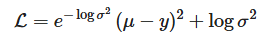
While this approach theoretically provides solutions to Problem 1 (predict target values) and Problem 2 (estimate confidence of predictions), it has limitations with respect to Problem 3: are these uncertainty estimates accurate? For example, the modeled noise is assumed to be Gaussian, an assumption that does not hold here (per our uniform noise), and may not hold in real-world applications. Moreover, error for μ and logσ2 are collectivelyA minimized per-sampleB. Concerning point A, if the model can reduce the squared error (μ−y)2 significantly (by fitting the mean well), the optimizer may push logσ2logσ2 toward negative values (i.e., very small variance) to further shrink the first term. Conversely, if errors remain large, the optimizer can inflate logσ2 to “explain away” residuals. For point B, since logσ2 is learned per sample (or per input), the model can potentially overfit the noise structure of the training data. It might predict small variances where training labels happen to align well and very large variances elsewhere, leading to poor generalization. Both cases can lead to variance estimates that don’t correspond to the true predictive uncertainty. Thus, relative to held-out sets, we must characterize our approximation of uncertainty and, ultimately, calibrate it.
The following PyTorch Lightning code constructs a probabilistic neural network (provided as part of the simple_uq package), the necessary PyTorch data loaders, and a PyTorch Lightning trainer to orchestrate the training process. Intimate understanding of these components is not necessary: at a high level, we are simply training a model that predicts a value and an indication of its confidence.
# Construct the probabilistic neural network
pnn = PNN(
    input_dim=1,
    output_dim=1,
    encoder_hidden_sizes=[32, 32],
    encoder_output_dim=32,
    mean_hidden_sizes=[],
    logvar_hidden_sizes=[],
)

# Train dataloader
train_dataloader = DataLoader(
    TensorDataset(
        torch.Tensor(X_train).reshape(-1, 1),
        torch.Tensor(y_train).reshape(-1, 1),
    ),
    batch_size=64,
    shuffle=True,
    num_workers=4,
    persistent_workers=True,
)

# Validation data loader
val_dataloader = DataLoader(
    TensorDataset(
        torch.Tensor(X_val).reshape(-1, 1),
        torch.Tensor(y_val).reshape(-1, 1),
    ),
    batch_size=64,
    shuffle=False,
    num_workers=4,
    persistent_workers=True,
)

# Testing data loader
test_dataloader = DataLoader(
    TensorDataset(
        torch.Tensor(X_test).reshape(-1, 1),
        torch.Tensor(y_test).reshape(-1, 1),
    ),
    batch_size=64,
    shuffle=False,
    num_workers=4,
    persistent_workers=True,
)

# Early stopping callback
early_stop_callback = EarlyStopping(
    monitor="validation_loss", patience=10, verbose=False, mode="min"
)

# Initialize the trainer
trainer = pl.Trainer(
    max_epochs=500,
    callbacks=[early_stop_callback],
    enable_progress_bar=False,
    log_every_n_steps=1,
)

# Fit the model
trainer.fit(pnn, train_dataloader, val_dataloader)

# Get test set results
test_results = trainer.test(pnn, test_dataloader)
You are using the plain ModelCheckpoint callback. Consider using LitModelCheckpoint which with seamless uploading to Model registry.
GPU available: True (mps), used: True
TPU available: False, using: 0 TPU cores
HPU available: False, using: 0 HPUs
| Name | Type | Params | Mode
---------------------------------------------
0 | encoder | MLP | 2.2 K | train
1 | mean_head | MLP | 33 | train
2 | logvar_head | MLP | 33 | train
---------------------------------------------
2.2 K Trainable params
0 Non-trainable params
2.2 K Total params
0.009 Total estimated model params size (MB)
8 Modules in train mode
0 Modules in eval mode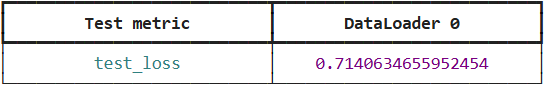
With our trained model, we can leverage the PNN implementation's get_mean_and_standard_deviation method to predict the mean and, instead of the network's typical log-variance output, the standard deviation. In other words, instead of the raw logσ2logσ2 output, this method outputs σσ. We'll do this for both the validation and test sets.
# Predict on val
y_val_pred_mean, y_val_pred_std = pnn.get_mean_and_standard_deviation(
    X_val.reshape(-1, 1)
)
y_val_pred_mean = y_val_pred_mean.flatten()
y_val_pred_std = y_val_pred_std.flatten()

# Predict on test
y_test_pred_mean, y_test_pred_std = pnn.get_mean_and_standard_deviation(
    X_test.reshape(-1, 1)
)
y_test_pred_mean = y_test_pred_mean.flatten()
y_test_pred_std = y_test_pred_std.flatten()
Visualizing the uncalibrated mean and standard deviation predictions of the test set, relative to the ground truth function, we get the following. Note that we multiply the standard deviation by 1.96 to construct a 95% confidence interval of the mean.
fig, ax = plt.subplots(figsize=(5, 3), dpi=150)

# Plot ground truth
ax.plot(
    ticks, ground_truth_function(ticks), ls="--", color="black", label="Ground truth"
)

# Plot predictions + uncertainty
ax.plot(X_test, y_test_pred_mean, label="Predictions")
ax.fill_between(
    X_test,
    y_test_pred_mean - 1.96 * y_test_pred_std,
    y_test_pred_mean + 1.96 * y_test_pred_std,
    alpha=0.2,
)

# Points
ax.scatter(
    X_test, y_test, s=8, alpha=1, label="Observations", color="k", facecolors="none"
)
ax.legend()
ax.set_xlabel("$x$")
ax.set_ylabel("$y$")

plt.show()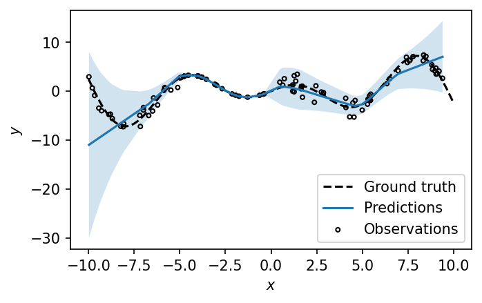
As expected, the model reports high variance in regions with noisier observations, and vice versa in low-variance regions. The bands here make intuitive sense, but we must investigate what proportion of our predictions fall within the observed error distribution. To this end, we can generate an average uncertainty calibration plot, as follows.
# Plot calibration
fig, ax = plt.subplots(dpi=150)
ax = uct.viz.plot_calibration(y_test_pred_mean, y_test_pred_std, y_test, ax=ax)
ax.get_lines()[0].set_color("black")
plt.show()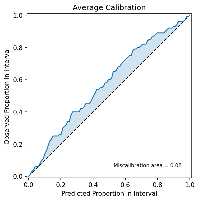
But what, exactly, is this plot showing us? From our standard deviation predictions, we can compute prediction intervals at different nominal coverage levels (e.g. 0.1, 0.2,..., 1.0). For example, with a 0.9 prediction interval, the model "claims" that “90% of true outcomes should fall inside this interval.” In the above plot, one can think of the x-axis (predicted proportion in interval) as this nominal coverage level, or what the model claims should be true. The y-axis (“observed proportion in interval”) is the empirical coverage, or the fraction of observed outcomes actually fell inside those intervals. Their mismatch is represented as deviations from the line y=x. In this example, we predict that ~20% of our predicted means fall within their accompanying predicted standard deviations. In reality, ~25% of observations actually fall within the predicted bounds. This suggests that our model is underconfident, overestimating its uncertainty for this task. Conversely, area below the line y=x would be indicative of overconfidence, or underestimation of its uncertainty.
To address this miscalibration, we can scale our predicted standard deviations such that predicted intervals more closely match observed intervals. But because we are fitting a scaling factor, it is important to ensure we aren't cheating in our correction. Similar to overfitting when training a machine learning model, we risk a poor result when calibrating to already-seen data. Thus, we will calibrate to a validation split, and evaluate on a fully held out test split.
# Train a scale-factor model
scale_factor = uct.recalibration.optimize_recalibration_ratio(
    y_val_pred_mean, y_val_pred_std, y_val, criterion="miscal"
)
# Plot scale factor result
fig, ax = plt.subplots(dpi=150)
ax = uct.viz.plot_calibration(
y_test_pred_mean, scale_factor * y_test_pred_std, y_test, ax=ax
)
ax.get_lines()[0].set_color("black")
plt.show()
We observe improved miscalibration area, and more importantly a centering of the distribution of uncertainty mischaracterization (previously all uncertainty predictions were underconfident, overestimating prediction intervals). Remember also that we calibrated our uncertainties on the validation set, but here are plotting the average calibration of the test set. This is a rough indication that our calibration does generalize in this case.
CYP3A4 Activity Prediction (OpenADMET)
As part of our mission, we've made training ADMET models as easy as possible (to the best of our ability) with anvil, an application programming interface (API) and command line interface (CLI) facilitating end-to-end ADMET modeling. This includes data ingestion, splitting, featurization, training, evaluation, and inference, all enabled for an ever-growing library of model types.
As part of the training process, we currently support uncertainty estimation through ensembling: that is, a suite of models is trained on randomly bootstrapped subsets of the training set, resulting is ostensibly distinct outputs from each ensemble member. At inference, ensemble predictions are averaged to yield a mean prediction, and the standard deviation is taken across predictions as our measure of uncertainty.
In practice, this all occurs under the hood automatically when specifying an ensemble for model training. Below we reproduce the relevant sections of the YAML configuration to train an ensemble of LGBM (light gradient-boosted machine) models, invoked with openadmet anvil --recipe-path lgbm.yaml. For a full configuration, see our docs and canonical recipes.
In the first section (model), we specify LGBM as the base model. We choose LGBM not necesarily as the most performant (though they can be quite effective), but as easily trainable on limited resources, e.g. a laptop.
In the ensemble section, we currently only support use of a CommitteeRegressor, though classification and other types of ensembling will eventually be supported. We semi-arbitrarily select n_models=5, and choose calibration_method="scaling-factor".
Committee regressor: an ensemble model made up of multiple regression models (“committee members”) whose predictions are combined, typically by averaging, to produce a final output.
Next, the split section must be configured to ensure we have distinct holdouts for validation and test. While LGBMs and other classic ML-style models don't strictly require a validation set for training, like in deep learning, the validation is used after training to calibrate uncertainties. Uncertainty calibration is then evaluated on the test set, generating metrics and an average calibration plot (configured in the report section).
We then simply call anvil, directing it to the workflow specification and output directory. As to not crowd the notebook, we're going to pipe stderr and stdout to a log file (i.e. &> log.txt) and tail the last line of the output to ensure the workflow is successful.
# Remove any existing runs
!rm -rf output

# Execute the workflow
!openadmet anvil --recipe-path lgbm.yaml --output-dir output &> log.txt

# Check the last line of the log
!tail -n 1 log.txt
Workflow completed successfully
We'll then inspect how we did in predicting CYP3A4 activity, with actual values on the x-axis and predicted values on the y-axis. This figure is generated by the workflow, so we load it in via Markdown.
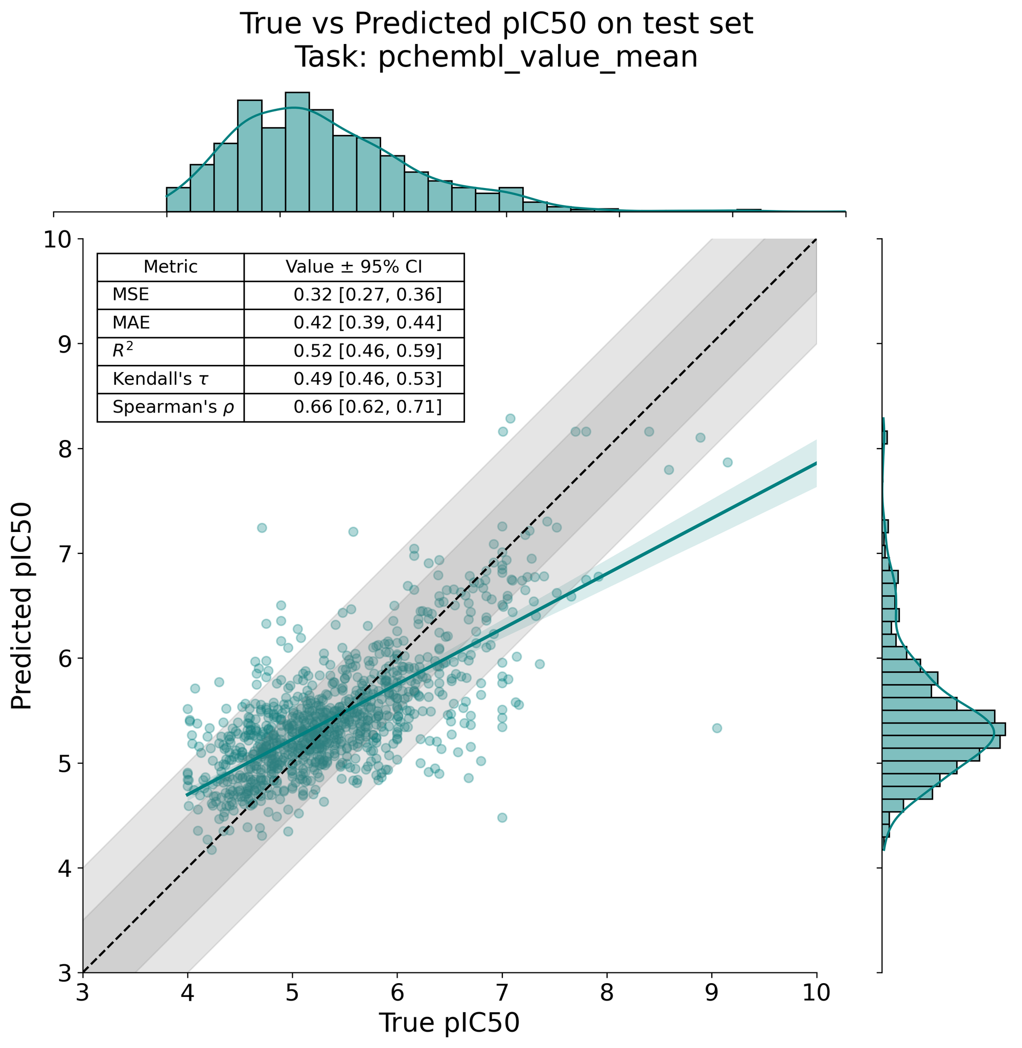
While not great, we have to remember that our dataset is fairly limited (N=4800), and that our base model has limited utility in representing such a difficult prediction task. More performant models, such as CheMeleon, a deep-learning foundation model that considers the graph representation of input molecules. Expect training times to increase substantially relative to LGBMs, though, especially without a GPU.
Finally, we'll take a look at the calibration result on the test holdout. Again, this plot is automatically generated by the workflow, we simply need to read it in.
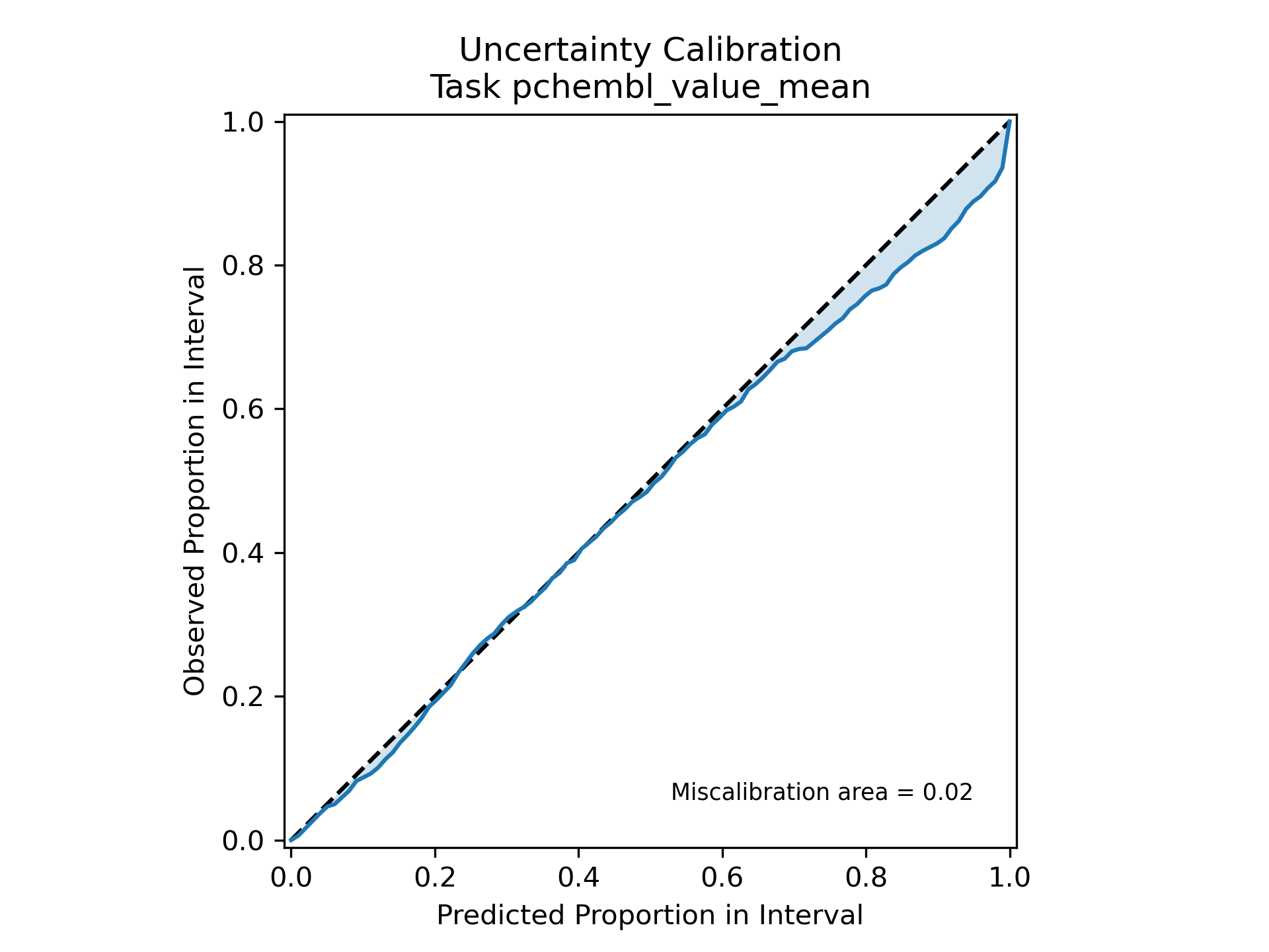
Our calibration result is impressive, indicating excellent agreement between predicted and actual uncertainties. Since we calibrate on a separate set than we test on, there's a reasonable indication that the calibration generalizes as well. But, while the calibration result is impressive, the actual uncertainty is... not so much. Plotting a distribution of uncertainty values on the test set gives:
fig, ax = plt.subplots(figsize=(6, 4), dpi=150)
sns.histplot(y_test_pred_std, bins=15, kde=True, ax=ax, stat="density", label="KDE")
median = np.median(y_test_pred_std)
ax.axvline(median, color="red", ls="--", label=f"Median={median:.2f}")
ax.set_xlabel("Predicted Uncertainty (pIC50)")
plt.legend()
plt.show()
The median predicted uncertainty is 1.50 pIC50 units, which is about 5 times higher than typical experimental error (~0.3 log units). Some compounds in the test set have high enough uncertainty to cover the entire range of possible values! While we certainly did not solve CYP3A4 inhibition prediction, the result can still be useful. We can interrogate why some predictions have such high uncertainty and, assuming access to experimental assays, run said uncertain compounds to improve the model. Of course, this is from the test set, so we already know the pIC50 values. In theory, we can imagine if these were true unknowns and the utility of assaying highly uncertain compounds.
Where do we go from here?
For our ADMET predictions, implications in downstream active learning are of particular relevance. In active learning, new data points are selected not just based on the model’s predictions, but also on how uncertain those predictions are. In some applications, we explicitly target areas where the model is least confident to maximize learning efficiency. In others, we balance high-valued predictions and uncertainty, e.g. to simultaneously identify potent ligands and to improve next-iteration model performance. If uncertainties are poorly calibrated, the model may either overlook informative samples (if underconfident) or waste resources on uninformative ones (if overconfident), ultimately reducing the effectiveness of the active learning process. Proper calibration enables more reliable decision-making (molecule selection) and accelerates model improvement.
We hope you take away the importance of uncertainty calibration in machine learning, using examples from the Uncertainty Toolbox and OpenADMET. We showed how uncalibrated models can misrepresent confidence, and how simple scaling can improve reliability. Finally, we outlined how OpenADMET automates uncertainty estimation and calibration for ADMET predictions, making model outputs more trustworthy and actionable.